from waveforms to speaker classification
introduction
sound is one of the most information-rich signals we encounter. a single audio recording encodes pitch, timbre, rhythm, loudness, and spatial cues, all riding on pressure variations that oscillate thousands of times per second. unlocking that information requires tools from signal processing, statistics, and data science working in concert.
this article walks through three practical applications that span the audio processing pipeline end to end: simulating how a cochlear implant transforms speech, synthesizing a piano-and-drums arrangement from scratch, and classifying speakers using spectral features and machine learning. each example is drawn from the audiosigpy project, a compact python library built for exploration and experimentation with sound. along the way we will encounter fourier transforms, filterbanks, perceptual frequency scales, peak detection, and more. these form the core toolkit that bridges raw waveforms and higher-level analysis.
part 1: hearing, simulating auditory experience
stereo separation and the cocktail party problem
the simplest demonstration of audio signal structure is stereo panning. given two mono tracks (say, a vocal line and an instrumental) you can assign one to the left channel and the other to the right:
data = np.hstack([vocal.get_signal_data()[:N], music.get_signal_data()[:N]])
wf_left = asp.Waveform("Left Vocals")
wf_left.set_signal_data(data=data, sample_rate=fs)
swap the column order and the vocal switches ears. this is trivial from a coding perspective, but it models a real phenomenon: our auditory system exploits interaural differences to separate simultaneous sound sources. stereo separation is the foundation of spatial audio, language-learning tools, and karaoke systems alike.
modeling hearing loss with audiograms and filterbanks
real hearing loss is frequency-dependent. a "noise-exposed" listener might have near-normal sensitivity below 2 khz but a sharp notch around 4 khz, the classic noise-induced dip. a "sensorineural loss" pattern shows a more gradual roll-off toward high frequencies. these patterns are captured in an audiogram: a plot of hearing thresholds (in db) across frequency.
to simulate the experience, audiosigpy's Processor class decomposes audio into 22 frequency bands using a butterworth bandpass filterbank spaced on the equivalent rectangular bandwidth (erb) scale:
deaf_proc = asp.Processor(band_count=22, scale="erb")
streams, _ = deaf_proc.filterbank(signal=data[:, channel], sample_rate=fs)
each band's energy is then attenuated according to the audiogram threshold for that frequency. the result is reassembled into a single waveform. listeners hear a version of the original audio with the frequency-specific deficits that a person with that hearing profile would experience.
the signal processing chain:
- bandpass filtering: a 2nd-order butterworth filter isolates each frequency band.
- sound pressure level (spl) measurement:
calc_spl()computes rms energy in decibels:SPL = 20 * log10(RMS / p_ref), wherep_ref = 2 * 10^-5pa is the standard reference pressure. - level transformation:
spl_transform()scales each band's energy to match the attenuated target. - reconstruction: the modified bands are summed back into a time-domain signal.
the erb scale deserves special attention. unlike a linear frequency axis, erb spacing approximates the bandwidth of the human auditory filters: narrower at low frequencies where pitch discrimination is fine, wider at high frequencies. this perceptual grounding makes erb-spaced filterbanks a natural choice for any application that aims to model human hearing.
the cochlear implant processor
a cochlear implant (ci) bypasses damaged hair cells in the inner ear and stimulates the auditory nerve directly with electrical pulses. the implant's external processor must compress the full auditory spectrum into a small number of electrode channels, typically 22. audiosigpy's Cochlear class implements a simplified version of this pipeline:
ci = asp.Cochlear()
prep_signal = ci.process(signal=data, sample_rate=fs)
true_signal = ci.signal(signal=prep_signal, sample_rate=fs)
sim_signal  = ci.simulate(signal=prep_signal, sample_rate=fs)
the process() method orchestrates six stages:
- filterbank decomposition: the input is split into 22 erb-spaced bands using butterworth bandpass filters.
- rectification: each band is full-wave rectified (absolute value), converting the ac audio signal into a dc envelope. this is analogous to the biological conversion from mechanical vibration to neural firing rate.
- envelope extraction: a lowpass butterworth filter (cutoff around 300 hz) smooths each rectified band, capturing the slow-varying amplitude contour that carries speech information.
- energy normalization: rms-based gain correction ensures that the processing chain doesn't distort relative energy levels between bands.
- current steering: because the number of analysis bands may differ from the number of output electrodes, energy must be redistributed. the
steer()method computes a mapping matrix in log-frequency space, proportionally routing energy from analysis bands to electrode nodes. - balancing: a gamma-distribution-shaped curve adjusts the energy profile across electrodes, compensating for the uneven perceptual sensitivity of the auditory nerve at different positions along the cochlea.
the signal() method then modulates a carrier (a sine or pulse wave at a fixed frequency) with these envelopes, mimicking the electrical stimulation pattern. the simulate() method does something different: it assigns each electrode a carrier at its corresponding center frequency (optionally compressed to a narrower range), then sums the modulated carriers. this produces an acoustic signal that a normal-hearing listener can play through headphones to get an impression of what a ci user hears.
comparing the spectrograms of the original speech, the "true" electrical signal, and the simulated acoustic signal reveals the dramatic information compression: fine spectral detail is replaced by coarse energy contours across a handful of channels. yet speech remains intelligible, a testament to the redundancy of the speech signal and the brain's ability to extract meaning from sparse cues.
part 2: music, sound synthesis from first principles
frequency modulation synthesis
the music notebook begins with a frequency modulation (fm) synthesis example inspired by the supercollider audio programming language. the idea is simple in principle but rich in output: use one oscillator (the "modulator") to vary the frequency of another (the "carrier").
# Low-frequency control oscillators at 1 Hz and 3 Hz
sine_control = [asp.sine(frequency=f, duration=1, sample_rate=44100) for f in [1, 3]]
# Exponential scaling from 100 Hz to 2000 Hz
exp_control = np.mean([100 * (2000/100) ** ((sc + 1) / 2) for sc in sine_control], axis=0)
# Carrier oscillator with time-varying frequency
audio_wave = asp.choose_generator(duration=None, name="sine", args={
    "frequency": exp_control, "sample_rate": 44100, "phase": 0, "amplitude": 0.2
})
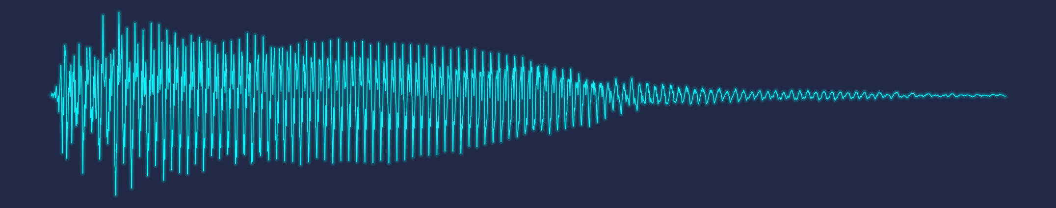
the sine() generator in audiosigpy accepts either a scalar frequency or an array of instantaneous frequencies, one value per sample. when the frequency input itself is a sinusoid, the result is fm synthesis: a single line of code produces the shimmering, evolving timbres that defined early digital synthesizers.
the choose_generator() gateway function dispatches to any of eight waveform types (sine, square, triangle, sawtooth, pulse, white noise, chirp, glottal) through a unified interface. this pattern keeps the api clean while supporting diverse synthesis needs.
additive synthesis: building a piano tone from its harmonics
a more analytical approach to synthesis starts with a real recording. the notebook loads a c4 piano sample and computes its magnitude spectrum via calc_spectra(), which internally runs an fft and extracts the magnitude and phase components:
_, mag_sp, _ = asp.calc_spectra(signal=wf.get_signal_data(), clip=True)
freqs = wf.frequency_series(clip=True)
peaks = asp.find_peaks(signal=mag_sp, height=500)[0]
the find_peaks() function identifies prominent spectral peaks, the harmonic partials that give the piano its characteristic timbre. each peak's frequency and relative magnitude are extracted, and a set of sine waves at those frequencies and amplitudes is summed to produce a synthetic approximation:
for i in range(len(frequencies)):
    signal = asp.sine(frequency=frequencies[i], duration=1, amplitude=magnitudes[i])
    signals.append(signal)
complex_signal = np.hstack(signals).sum(axis=1).reshape((-1, 1))
window = asp.choose_window(complex_signal.shape[0], "tukey")
complex_signal *= window
the tukey window applied at the end tapers the signal's onset and offset, preventing the audible clicks that would result from an abrupt start or stop. this is additive synthesis in its purest form: any complex timbre can be approximated by a weighted sum of sinusoids, as fourier's theorem guarantees.
the talkbox effect: cross-synthesis with filterbanks
the talkbox is a classic audio effect where the spectral envelope of one signal (the "modulator", typically speech) is imposed on the frequency content of another (the "carrier", typically a guitar or synth). audiosigpy implements this as a Talkbox processor:
talkbox = asp.Talkbox()
talkbox_mod = talkbox.process(signal=modulator.get_signal_data()[:, 0], sample_rate=fs)
talkbox_signal = talkbox.signal(carrier=carrier.get_signal_data()[:, 0],
                                modulator=talkbox_mod, sample_rate=fs)
the process() method extracts the modulator's spectral envelope through the same filterbank-rectify-envelope-normalize pipeline used in the cochlear implant processor. the signal() method then decomposes the carrier through its own filterbank and multiplies each carrier band by the corresponding modulator envelope. the result: the carrier's raw harmonic content is sculpted into the vowel shapes and consonant transients of speech. the guitar "talks."
this is an elegant demonstration of how the same signal processing primitives (bandpass filtering, envelope extraction, multiplication) serve radically different applications depending on context.
full music generation: piano and drumset synthesizers
the most ambitious example generates a complete musical arrangement of "bella ciao" with piano and drums. the Piano class extends Synthesizer to accept a data dictionary encoding musical notation:
bella_ciao = {
    "base_unit": 1/8,
    "notes": [11, 4, 6, 11, 4, 6, 7, ...],     # Note IDs (C=0, C#=1, ..., B=11)
    "octaves": [4, 5, 5, 4, 5, 5, 5, ...],       # Octave numbers
    "durations": [1, 1, 1, 0.5, 0.5, ...],        # Beat durations
    "beats": [5, 6, 7, 7.8, 8, ...],              # Beat positions
    "amplitudes": [p] * len(notes),                # Dynamic levels
    "tempos": [120] * len(notes),                  # BPM
}
the note-to-frequency conversion uses note2frequency(), which maps note ids and octave numbers to hz values via the standard equal-temperament formula. the Synthesizer base class provides the building blocks: oscillator() for tone generation, envelope() for exponential amplitude shaping (attack and decay), noise() for filtered white noise, resonator() for bandpass reinforcement of specific frequency bands, and smooth() for final polish.
the Drumset class synthesizes percussion from first principles:
- kick drum: a low-frequency oscillator (60-120 hz) with rapid exponential decay, plus a noise burst filtered through resonant bands for the characteristic "thump" and "click."
- snare drum: filtered white noise through mid/high-frequency resonant bands, combined with a 150 hz tonal component, shaped by an exponential envelope.
- hi-hat / crash cymbal: high-frequency filtered noise with very short or sustained envelopes respectively.
each drum hit is synthesized as an independent signal, placed at the correct beat position, and summed with the piano track:
piano_track = piano.process(data=bella_ciao)
drum_track = drumset.process(data=bc_drum)
new_signal = np.zeros((int(duration * piano_track.get_sample_rate()), 1))
new_signal[:drum_track.get_sample_count()] = drum_track.get_signal_data() / 4
new_signal[-piano_track.get_sample_count():] += piano_track.get_signal_data()
the result is a complete synthetic rendition of a recognizable tune, generated entirely from mathematical functions, without any audio samples.
part 3: speech, from spectral features to speaker classification
edge detection for speech activity
before analyzing speech content, you need to know where speech occurs in a recording. audiosigpy's find_endpoints() function implements a dual-threshold approach based on two complementary signal properties:
- short-time energy (intensity): speech is louder than silence. rms energy computed over short windows provides a robust activity indicator.
- zero-crossing rate (zcr):
calc_zcr()counts how often the signal crosses the zero axis per unit time. unvoiced speech (fricatives like "s" and "f") has high zcr, while voiced speech and silence have lower rates.
by applying thresholds on both metrics simultaneously, the algorithm identifies speech regions while rejecting isolated noise bursts that might trigger a single detector.
endpoints = asp.find_endpoints(
    signal=data, sample_rate=fs,
    int_threshold=40, zcr_threshold=0.05
)
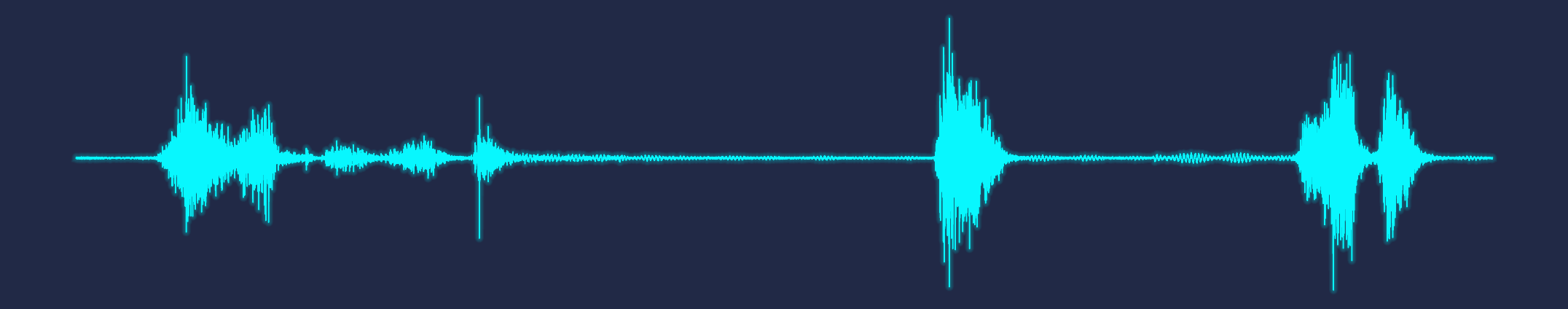
the notebook demonstrates this on speech samples from biden and trump during the 2024 presidential debate, producing clean segmentation that isolates speech from inter-utterance silence.
extracting a spectral feature vector
with speech segments isolated, the next step is to characterize each speaker's voice quantitatively. the notebook computes a rich feature vector for each audio segment:
acoustic energy features:
- sound pressure level (spl):
calc_spl()provides a calibrated db measure of overall energy:SPL = 20 * log10(RMS / 2e-5). - perceptual loudness (lufs):
calc_loudness()uses thepyloudnormlibrary to compute loudness according to the itu-r bs.1770 standard, which applies frequency weighting that models human sensitivity. both normalized and raw values are captured.
spectral shape features:
- centre of gravity:
calc_centre_gravity()computes the weighted mean frequency of the spectrum, indicating whether energy is concentrated at low or high frequencies. a deep voice has lower spectral center of gravity than a bright one. - standard deviation:
calc_std()measures the spectral spread around the center of gravity. - skewness:
calc_skewness()quantifies asymmetry in the spectral distribution. a positive skew means energy is concentrated below the mean with a long high-frequency tail. - kurtosis:
calc_kurtosis()measures the "peakedness" of the spectrum. high kurtosis indicates energy concentrated in a narrow frequency range; low kurtosis indicates a flat, broad spectrum.
pitch features:
- fundamental frequency (f0): rather than using the
pitch_contour()function (which tracks f0 over time), the notebook takes a frequency-domain approach. it computes the magnitude spectrum via fft, detects peaks withfind_peaks(), filters to the typical human f0 range (below 250 hz), and selects the dominant peak. this gives a single representative pitch value per segment.
_, mags, _ = asp.calc_spectra(signal=data, clip=True)
peaks = asp.find_peaks(signal=mags, height=1)[0]
mags, freqs = mags[peaks], freqs[peaks]
mask = (freqs < 250) & (mags > 80)
pitch = freqs[np.argsort(mags[mask], axis=0)[-1]]
the resulting feature matrix has 73 rows (37 biden segments + 36 trump segments) and 10 numeric columns, a compact but informative representation of each speech sample.
correlation analysis: what the features reveal
a correlation heatmap reveals the internal structure of the feature space:
- strong positive correlations: centre of gravity and standard deviation move together (broader spectra have higher centers). skewness and kurtosis are tightly linked (both reflect spectral concentration).
- strong negative correlations: skewness inversely tracks centre of gravity and loudness. louder, brighter speech tends to have more symmetric spectra.
- weak correlations: duration shows little relationship with any spectral feature, suggesting that segment length doesn't systematically bias the acoustic measurements.
a pairplot colored by speaker shows visible separation on several feature axes, particularly pitch, spectral center of gravity, and loudness, suggesting that classification is feasible.
unsupervised classification: kmeans clustering
the first modeling approach is unsupervised. after standardizing features with StandardScaler, kmeans with k=2 is applied:
kmeans = KMeans(n_clusters=2, n_init=10, random_state=0)
kmeans.fit(X_scaled)
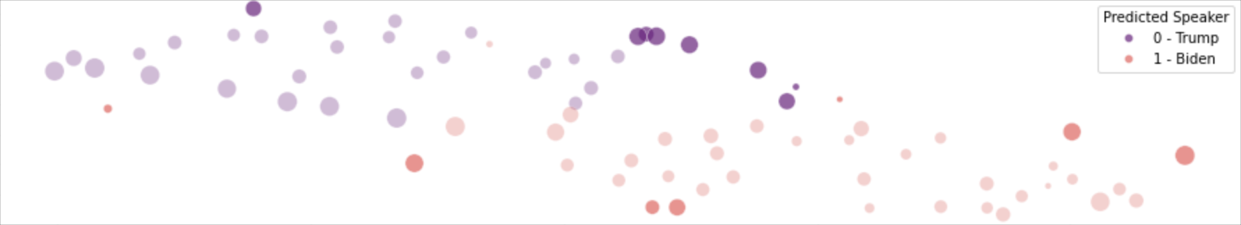
umap projection visualizes the cluster structure in 2d, revealing two reasonably distinct groups. performance metrics against the true speaker labels:
| metric | score |
|---|---|
| silhouette score | 0.35 |
| adjusted rand index | 0.60 |
| precision | 0.87 |
| sensitivity (recall) | 0.92 |
| specificity | 0.86 |
| f1 score | 0.89 |
an f1 of 0.89 from a completely unsupervised method is notable. it confirms that the spectral features extracted by audiosigpy capture genuine acoustic differences between speakers, differences large enough to emerge without any labeled training data.
supervised classification: logistic regression
a logistic regression model trained on 80% of the data and tested on the remaining 20% improves on kmeans:
| metric | train | test |
|---|---|---|
| precision | 0.94 | 0.86 |
| sensitivity | 0.97 | 1.00 |
| specificity | 0.93 | 0.89 |
| f1 score | 0.95 | 0.92 |
the test set achieves perfect sensitivity (every biden segment correctly identified) with an f1 of 0.92. the slight precision drop indicates occasional misclassification of trump segments, consistent with the fact that some acoustic features overlap between speakers.
the umap projections show that the logistic regression decision boundary cleanly separates the two speakers in the projected feature space, with train points (faded) and test points (bright) both falling on the correct side.
what this tells us about speech signals
the success of these classifiers, especially the unsupervised one, underscores a key insight: speech signals carry speaker identity information in their long-term spectral statistics. features like centre of gravity, spectral spread, and pitch are shaped by the physical properties of each speaker's vocal tract (its length, shape, and resonance characteristics) and habitual speaking patterns (loudness, intonation). these properties are stable enough across utterances to support reliable classification even with a small dataset and simple models.
the signal processing toolkit behind it all
what makes these diverse applications possible from a single library is a layered architecture of reusable primitives:
layer 1: array and validation infrastructure
the array.validate() function is called at the entry point of nearly every operation. it coerces inputs to numpy arrays, ensures consistent dimensionality (at least 2d), aligns multi-channel data, and catches type errors early. this small piece of infrastructure eliminates an entire class of bugs that plague audio processing code.
layer 2: signal generation
eight waveform generators (sine, square, triangle, sawtooth, pulse, white_noise, chirp, glottal) provide the raw material for synthesis. critically, most accept array-valued frequency parameters, enabling frequency modulation and time-varying synthesis in a single function call.
layer 3: spectral analysis
the dft() function implements the discrete fourier transform from the mathematical definition. it's useful for understanding, though too slow for practical use at O(N²). the fft() function provides both an educational recursive cooley-tukey implementation and a stable numpy-backed version. stft() and istft() handle time-frequency analysis via the short-time fourier transform, producing the spectrograms that are central to audio visualization.
layer 4: window functions
fourteen window functions (hann, hamming, blackman, kaiser, gaussian, tukey, and more) are available through the choose_window() gateway. windows are essential for reducing spectral leakage in stft analysis and for shaping the onset/offset of synthesized sounds.
layer 5: filtering
butterworth iir filters (butter_filter()), fir filters (fir_filter()), gammatone auditory filters (gamma_tone_filter()), and convolution (convolve()) provide the tools to isolate, shape, and transform frequency content. the filterbank pattern (decompose a signal into bands, process each independently, recombine) appears in the cochlear implant processor, hearing loss simulator, and talkbox effect.
layer 6: acoustic metrics and statistics
functions like calc_rms(), calc_spl(), calc_loudness(), calc_zcr(), calc_centre_gravity(), calc_skewness(), and calc_kurtosis() transform raw signals into interpretable scalar features. these are the bridge between signal processing and data science, the point where a time-series waveform becomes a row in a feature matrix suitable for machine learning.
layer 7: perceptual frequency scales
the erb (equivalent rectangular bandwidth) scale conversions (hz2erb_rate(), erb_rate2hz(), erb_centre_freqs()) and musical note conversions (note2frequency(), frequency2note()) connect raw hz values to human perception. the erb scale is critical for the hearing simulations; musical note conversion is central to the piano synthesizer.
layer 8: high-level classes
Waveform, Processor (with Cochlear and Talkbox subclasses), and Synthesizer (with Piano and Drumset subclasses) compose the lower-level primitives into task-specific workflows. each class encapsulates a multi-step processing chain while remaining configurable through its constructor parameters.
lessons and takeaways
1. the same primitives serve many masters. filterbanks, envelope extraction, and carrier modulation appear in hearing simulation, talkbox effects, and drum synthesis. mastering these building blocks opens a wide range of applications.
2. perceptual scales matter. linear frequency axes are mathematically convenient but perceptually misleading. the erb scale, which models the frequency resolution of the human ear, produces more meaningful filterbanks for any application involving human listening.
3. spectral features are powerful representations. a handful of statistics computed from the frequency-domain representation of speech (center of gravity, spread, skewness, kurtosis, pitch) carry enough information to distinguish speakers with high accuracy. this is the foundation of speaker recognition, emotion detection, and many other speech analytics tasks.
4. unsupervised methods can surprise you. kmeans clustering on spectral features achieved 89% f1 without seeing any labels. when the underlying signal structure is strong, you don't always need labeled data to find it.
5. synthesis is analysis in reverse. building a piano tone from its detected harmonics, or a drum hit from noise and resonance, reinforces understanding of what analysis reveals. there is no better way to internalize the fourier transform than to hear the result of summing sinusoids at the frequencies and amplitudes your fft measured.
conclusion
audio signal processing sits at a productive intersection of physics, mathematics, perception, and computation. the examples explored here (hearing simulation, music synthesis, and speaker classification) demonstrate how a shared foundation of signal processing techniques connects domains that might seem unrelated on the surface. a cochlear implant processor and a talkbox effect use the same filterbank-envelope-modulation pipeline. the spectral analysis that reveals a piano's harmonics also generates the features that distinguish one speaker from another.
for data scientists, the key takeaway is that domain-specific feature engineering, grounded in the physics of sound and the psychoacoustics of hearing, dramatically outperforms generic approaches. the spectral statistics used for speaker classification aren't arbitrary; they capture the physical properties of the vocal tract. the erb-spaced filterbanks used in hearing simulation aren't a convenience; they model the actual frequency resolution of the human ear.
understanding these connections transforms audio from an opaque blob of samples into a structured, analyzable, and synthesizable signal. and that understanding is where the real fun begins.
built with audiosigpy by w. jonas reger.